Reading Measurements Against Catalog Specs - 1
This post is part of my series on High Performance Computing.
What this post covers
This post is mainly about what you should think about when you look at experimental data. You need this to judge whether a measurement is valid. I’ll go through how to check whether a measured number is really what it should be by comparing it with the catalog specs on the datasheet.
Hardware specs
| Machine | NVIDIA GH200 |
| CPU FP32 FLOPS | 7.1 TFLOPS (calculated) |
| CUDA FP32 FLOPS | 67 TFLOPS |
| Tensor Core FP32 FLOPS | 494 TFLOPS |
| CPU Memory Bandwidth | Up to 512GB/s |
| GPU Memory Bandwidth | 4.0 TB/s |
Reasoning from the hardware specs
To keep things simple, the discussion below uses matrix multiplication. Given square matrices $A, B, C \in \mathbb{R}^{N \times N}$, consider the product
\[C = AB\]For $N = 512$, here are the results for a naive matmul, NumPy’s matmul, PyTorch’s matmul, and PyTorch’s matmul using Tensor Cores. Everything is FP32, and the code is in Materials (run it with run_all.sh).
| Method | Time (ms) |
|---|---|
| CPU (Naive) | 93.81 |
| CPU (Numpy) | 1.576e-01 |
| GPU (Non Tensor Core) | 1.723e-02 |
| GPU (Tensor Core) | 1.304e-02 |
So what can we tell from these results? First, the naive CPU code is the slowest. It’s simple code that even a freshman who just started programming could write; it looks like the code below. I won’t cover it in this post, but the other methods get their speed from techniques like loop unrolling, tiling, SIMD, shared memory and Tensor Cores.
void matmul(int n, const float *A, const float *B, float *C) {
    for (int i = 0; i < n; i++)
        for (int j = 0; j < n; j++) {
            float sum = 0.0f;
            for (int k = 0; k < n; k++) sum += A[i * n + k] * B[k * n + j];
            C[i * n + j] = sum;
        }
}
Now for the main topic. CPU (Numpy) certainly looks faster than the naive CPU matmul. But is this result optimal? In other words, does it get enough performance out of the hardware?
| Method | Time (ms) |
|---|---|
| CPU (Naive) | 93.81 |
| CPU (Numpy) | 1.576e-01 |
| GPU (Non Tensor Core) | 1.723e-02 |
| GPU (Tensor Core) | 1.304e-02 |
One yardstick is to compare against the theoretical FLOPS. A matmul takes $2N^3$ FLOPs, so the achieved FLOPS are
| Method | Time (ms) | GFLOPS |
|---|---|---|
| CPU (Naive) | 93.81 | 2.86 |
| CPU (Numpy) | 1.576e-01 | 1704 |
| GPU (Non Tensor Core) | 1.723e-02 | 15576 |
| GPU (Tensor Core) | 1.304e-02 | 20584 |
The naive CPU matmul reaches only 0.040% of the CPU’s theoretical 7.1 TFLOPS, so it’s fair to say it isn’t using the hardware. What about the others? Are they getting the performance out of the hardware? At this point most people would probably say no: CPU (Numpy) reaches 24% of 7.1 TFLOPS, GPU (Non Tensor Core) 23% of 67 TFLOPS, and GPU (Tensor Core) only 4.2% of 494 TFLOPS. Why is that? Are NumPy and PyTorch actually poorly optimized?
Roofline
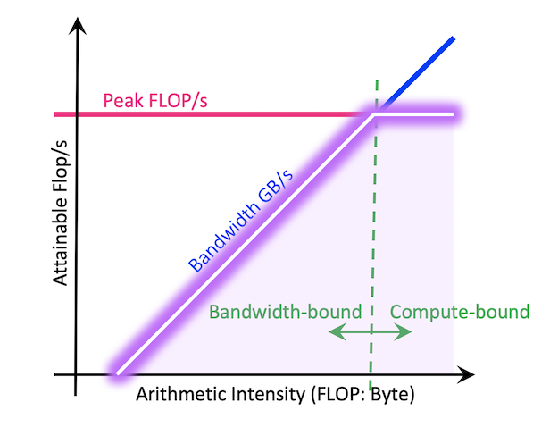 Image from NERSC Documentation [2]
The tool for answering that question is the Roofline model. The “theoretical FLOPS” in a catalog spec is what you get when the arithmetic units run nonstop. A real program, however, has to bring the data for those units in from memory, and if the data supply can’t keep up, the units sit waiting. The Roofline model [1] shows in a single figure whether performance is limited by how fast you compute or by how fast you move data.
The Roofline equations
First, define the following quantities.
- $W$ [FLOP]: the number of floating-point operations the program performs
- $Q$ [Byte]: the amount of data the program moves to and from memory (here, RAM)
- $P_{\mathrm{peak}}$ [FLOP/s]: the hardware’s theoretical FLOPS
- $B$ [Byte/s]: the hardware’s memory bandwidth
Computation takes at least $W / P_{\mathrm{peak}}$, and data transfer takes at least $Q / B$. Even if computation and transfer overlap perfectly, the run time $T$ can’t be shorter than the slower of the two.
\[T \geq \max\left(\frac{W}{P_{\mathrm{peak}}}, \frac{Q}{B}\right)\]Rewriting this in terms of achieved FLOPS $P = W / T$ gives
\[P \leq \min\left(P_{\mathrm{peak}}, \frac{W}{Q} \cdot B\right) = \min\left(P_{\mathrm{peak}}, I \cdot B\right)\]where
\[I = \frac{W}{Q} \quad [\mathrm{FLOP/Byte}]\]is called the arithmetic intensity: how many operations you perform per byte of data you bring in. That’s all there is to the Roofline model. If you plot $I$ on the horizontal axis and $P$ on the vertical axis, both log-scale, the upper bound is a diagonal line of slope 1 ($I \cdot B$) joined to a horizontal line ($P_{\mathrm{peak}}$), which looks like a roof. That’s where the name Roofline comes from.
The point where the two lines meet,
\[I^{*} = \frac{P_{\mathrm{peak}}}{B}\]is called the ridge point.
- A program with $I < I^{*}$ is memory bound. Faster arithmetic units won’t help; the bound is set by $I \cdot B$.
- A program with $I > I^{*}$ is compute bound. The bound is set by $P_{\mathrm{peak}}$.
So a measurement should be judged not against the theoretical FLOPS, but against the Roofline bound $\min(P_{\mathrm{peak}}, I \cdot B)$. Even if a memory-bound program reaches only 5% of the theoretical FLOPS, it’s getting the most out of the hardware if it’s close to $I \cdot B$.
The ridge point of GH200
Let’s compute the ridge points from the spec table at the top.
| Unit | $P_{\mathrm{peak}}$ | $B$ | $I^{*}$ [FLOP/Byte] |
|---|---|---|---|
| CPU (Grace, FP32) | 7.1 TFLOPS | 512 GB/s | 13.9 |
| GPU (CUDA Core, FP32) | 67 TFLOPS | 4.0 TB/s | 16.75 |
| GPU (Tensor Core, TF32) | 494 TFLOPS | 4.0 TB/s | 123.5 |
To be compute bound on Tensor Cores, you need 123.5 operations for every byte you read, or about 500 operations per FP32 value (4 bytes). Memory is very slow relative to the arithmetic units. This also explains why each new GPU generation puts so much weight on HBM bandwidth. And since algorithms that reuse each loaded value 100+ times are almost all matmul-like, you can see that most algorithms are memory bound.
Arithmetic intensity of matmul
Now let’s find the arithmetic intensity of $C = AB$. Each element of $C$ is a dot product of length $N$, with $N$ multiplies and $N$ adds, so
\[W = 2N^3\]The data transfer $Q$, unlike $W$, depends on the implementation and the cache size, so it isn’t uniquely determined. So when evaluating hardware performance, we consider a lower bound $Q_{\min}$ that no implementation can go below. Since $Q \geq Q_{\min}$, the arithmetic intensity has an upper bound $I \leq I_{\max} = W / Q_{\min}$, and the Roofline bound becomes $P \leq \min(P_{\mathrm{peak}}, I_{\max} \cdot B)$.
The simplest lower bound is that you must read $A$ and $B$ at least once and write $C$ at least once (compulsory traffic). In FP32 (4 bytes) that is
\[Q_{\min} \geq 3 \times 4N^2 = 12N^2 \quad [\mathrm{Byte}]\]and using only this bound,
\[I_{\max} = \frac{2N^3}{12N^2} = \frac{N}{6}\]From this alone, it looks as if the arithmetic intensity of matmul grows without limit as $N$ grows.
A lower bound from the red-blue pebble game
However, the $12N^2$ bound is achievable only when all three matrices fit in cache. When they don’t, data that was evicted from the cache has to be read back from DRAM. The question “how much data must move, at minimum, between a fast memory of capacity $M$ and an unlimited slow memory?” was formalized by Hong and Kung as the red-blue pebble game [3]. Red pebbles represent data in fast memory (cache), blue pebbles represent data in slow memory (DRAM), and at most $M$ red pebbles can be on the board at once. Under these rules, you ask for the minimum number of red↔blue swaps needed to finish computing the whole computation graph.
Hong and Kung showed that the data transfer of standard $O(N^3)$ matmul (excluding Strassen-like algorithms) is $\Omega(N^3 / \sqrt{M})$. Later, Smith et al. [4] gave a tight bound including constants: with $S$ words of fast memory, the transfer is asymptotically at least $2N^3 / \sqrt{S}$ words. Converting to bytes with $M$ [Byte] $= 4S$,
\[Q_{\min} \gtrsim \max\left(12N^2, \frac{16N^3}{\sqrt{M}}\right) \quad [\mathrm{Byte}]\]and the upper bound on arithmetic intensity is
\[I_{\max} \lesssim \min\left(\frac{N}{6}, \frac{\sqrt{M}}{8}\right) \quad [\mathrm{FLOP/Byte}]\]So the correct conclusion is that the arithmetic intensity of matmul does not grow without limit with $N$; it is capped by the cache size, $\sqrt{M}$. $N/6$ is only valid under the condition that all three matrices fit in cache. Optimizations such as tiling are about bringing the actual $Q$ close to this lower bound.
Estimating this for GH200: the GPU side (H100) has a 50 MB L2 cache, giving $\sqrt{M}/8 \approx 880$ FLOP/Byte, and the CPU side (Grace) has a 117 MB L3 cache, giving $\sqrt{M}/8 \approx 1350$ FLOP/Byte. Both are well above the ridge points (123.5 at most), so as far as DRAM traffic is concerned, GH200 can make large matmuls compute bound if the cache is used well. The same argument, however, applies at each level of the hierarchy, “L2 ↔ shared memory” and “shared memory ↔ registers”. Smaller levels have a smaller $\sqrt{M}$, so the bandwidth at each level can also become the bottleneck.
Now, when $N$ is small enough that all three matrices fit in cache, $I_{\max} = N/6$ applies as is. The matrix size that crosses the ridge point, $N^{*} = 6I^{*}$, is
| Unit | $I^{*}$ | $N^{*} = 6I^{*}$ |
|---|---|---|
| CPU (Grace, FP32) | 13.9 | 83 |
| GPU (CUDA Core, FP32) | 16.75 | 101 |
| GPU (Tensor Core, TF32) | 123.5 | 741 |
Revisiting the $N = 512$ results with Roofline
At $N = 512$, the three matrices total 3.1 MB, which fits easily in both the GPU’s L2 cache (50 MB) and Grace’s L3 cache (117 MB), so $I_{\max} = 512 / 6 \approx 85.3$ FLOP/Byte. The Roofline bounds are
- CPU: $\min(7.1\,\mathrm{T}, 85.3 \times 512\,\mathrm{G}) = 7.1$ TFLOPS (compute bound)
- GPU (Non Tensor Core): $\min(67\,\mathrm{T}, 85.3 \times 4.0\,\mathrm{T}) = 67$ TFLOPS (compute bound)
- GPU (Tensor Core): $\min(494\,\mathrm{T}, 85.3 \times 4.0\,\mathrm{T}) = 341$ TFLOPS (memory bound)
and the fraction of the Roofline bound achieved is shown below. I’ve been explaining all this with a lot of confidence, but it turns out NumPy and PyTorch’s regular FP32 kernel reach only 23–24%. I ran these experiments for the first time while writing this post, so this was a bit of a surprise.
| Method | GFLOPS | Roofline bound (GFLOPS) | Achieved |
|---|---|---|---|
| CPU (Numpy) | 1704 | 7100 | 24% |
| GPU (Non Tensor Core) | 15576 | 67000 | 23% |
| GPU (Tensor Core) | 20584 | 341000 | 6.0% |
Since $N = 512$ is smaller than $N^{*} = 741$, the Tensor Core case is memory bound and its bound drops to about 70% of the theoretical FLOPS (341 TFLOPS), yet it still reaches only about 6%. CPU (Numpy) and GPU (Non Tensor Core) also stay in the 20% range of their compute-bound limits. Roofline alone still doesn’t explain it.
Poor Tensor Core performance on small matmuls has also been raised as a problem in research. KAMI [5], presented at SC25, points out that while large GEMMs already run close to GPU peak performance, small and batched GEMMs still leave a lot of room for optimization. For small matrices, data exchange within a single thread block, that is, communication between registers and shared memory, limits performance. KAMI addresses this by bringing communication-avoiding (CA) matmul algorithms (1D/2D/3D), developed for distributed memory, inside a single GPU. It treats Tensor Cores as compute nodes, registers as local memory and shared memory as the communication channel, applying the transfer lower-bound argument above to each level of the memory hierarchy. You can see it as a concrete example of “the red-blue pebble game bound applies at every level of the hierarchy”.
What Roofline doesn’t show: fixed costs
Another factor Roofline doesn’t capture is fixed costs that don’t depend on problem size. On the GPU these include kernel launch (around 1–2 µs), PyTorch dispatch and synchronization; on the CPU, library call overhead and thread startup and synchronization (fork/join). Here I’ll just estimate the orders of magnitude.
At $N = 512$, putting the compute time $W / P_{\mathrm{peak}}$ and transfer time $Q_{\min} / B$ next to the measurements gives
| Method | Compute time | Transfer time | Measured | Difference ($T_0$) |
|---|---|---|---|---|
| CPU (Numpy) | 38 µs | 6.1 µs | 158 µs | ~120 µs |
| GPU (Non Tensor Core) | 4.0 µs | 0.79 µs | 17.2 µs | ~13 µs |
| GPU (Tensor Core) | 0.54 µs | 0.79 µs | 13.0 µs | ~12 µs |
On the GPU, compute and transfer take a few µs or less, yet the run takes over 10 µs. Moreover, the difference $T_0$ is about 12–13 µs for both FP32 and Tensor Cores, which shows a roughly constant cost that doesn’t depend on the arithmetic unit. The CPU likewise seems to carry a fixed cost on the order of 100 µs.
So consider a simple model with a fixed cost $T_0$:
\[T \approx T_0 + \max\left(\frac{W}{P_{\mathrm{peak}}}, \frac{Q}{B}\right)\]To reach 80% of the theoretical FLOPS in the compute-bound regime, you need $W / P_{\mathrm{peak}} \geq 4T_0$, that is,
\[2N^3 \geq 4 T_0 P_{\mathrm{peak}} \quad \Longrightarrow \quad N \geq \left(2 T_0 P_{\mathrm{peak}}\right)^{1/3}\]Plugging in the $T_0$ values above gives $N \approx 1200$ for CPU (Numpy), $N \approx 1200$ for GPU (Non Tensor Core) and $N \approx 2300$ for GPU (Tensor Core). The higher the theoretical FLOPS, the more work could have been done during the fixed cost, so hiding it takes a larger problem. $T_0$ isn’t really constant, so this is only an order-of-magnitude estimate, but it does show that “$N = 512$ is still too small to compare against the theoretical FLOPS”.
Achieved FLOPS across matrix sizes
Next, let’s look at measurements with varying $N$. The horizontal axis is the matrix size $N$, the vertical axis is achieved FLOPS, and the dotted lines are the theoretical FLOPS. You can see that the plots take a Roofline-like shape. During the experiments, the Claude Code I was using started optimizing the CPU matmul on its own, so I’ve included that result too: it’s CPU (NEON+OpenMP, 72 threads).
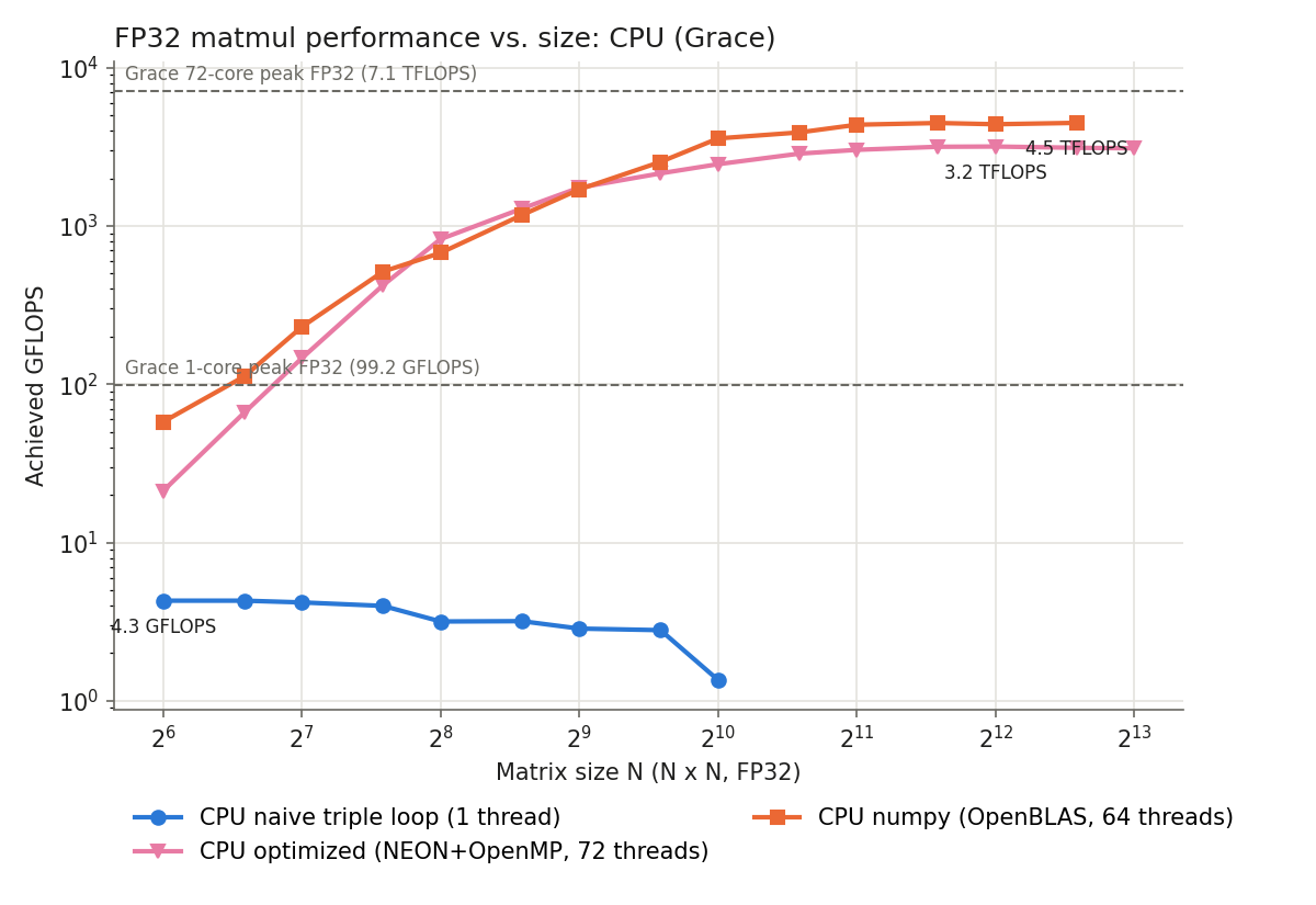
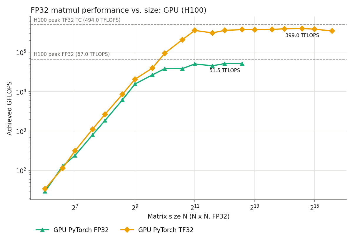
Every implementation gets faster as $N$ grows and eventually saturates. Comparing the saturated values with the theoretical FLOPS:
| Method | Max achieved FLOPS | Theoretical FLOPS | Achieved |
|---|---|---|---|
| CPU (Naive, 1 thread) | 4.3 GFLOPS | 99.2 GFLOPS (1 core) | 4.3% |
| CPU (NEON+OpenMP, 72 threads) | 3.2 TFLOPS | 7.1 TFLOPS | 45% |
| CPU (Numpy, OpenBLAS 64 threads) | 4.5 TFLOPS | 7.1 TFLOPS | 63% |
| GPU (PyTorch FP32) | 51.5 TFLOPS | 67 TFLOPS | 77% |
| GPU (PyTorch TF32) | 399 TFLOPS | 494 TFLOPS | 81% |
A few things stand out.
The GPU reaches about 80% of the theoretical FLOPS. GPU performance saturates around $N = 2^{11}$ for TF32 and around $N = 2^{10} \sim 2^{11}$ for FP32, which matches the order of the fixed-cost estimates above (about 2300 and 1200, respectively). For large enough $N$, the arithmetic intensity $N/6 \gg I^{*}$, so the workload is compute bound and the bound is the theoretical FLOPS. Even highly optimized libraries like cuBLAS almost never reach 100% of the theoretical FLOPS; 70–90% is a reasonable practical ceiling.
The naive implementation gets even slower at large $N$. The naive implementation reaches only about 4% of a single core’s theoretical 99.2 GFLOPS, and drops to 1.4 GFLOPS at $N = 2^{10}$. The innermost B[k * n + j] reads $B$ down a column with a stride of $4N$ bytes, so once the matrices no longer fit in cache, each 4-byte element costs a whole 64-byte cache line from memory. The actual $Q$ is then far larger than the lower bound $Q_{\min}$, and the actual arithmetic intensity is not $N/6$ but well below 1 FLOP/Byte. The naive implementation is a textbook memory-bound program, stuck on the diagonal line of the Roofline.
Summary
To judge whether a measurement gets the most out of the hardware, the following steps are a good way to think about it.
- From the operation count $W$ and the lower bound on data transfer $Q_{\min}$, find the upper bound on arithmetic intensity $I_{\max} = W / Q_{\min}$. If the data doesn’t fit in cache, also take the red-blue pebble game bound into account.
- From the catalog specs, find $I^{*} = P_{\mathrm{peak}} / B$ and decide whether the workload is memory bound or compute bound.
- Compare the measurement not with the theoretical FLOPS but with the Roofline bound $\min(P_{\mathrm{peak}}, I_{\max} \cdot B)$.
- If it’s far from the bound, check the implementation and improve it (though, of course, other factors may make further improvement impossible).
I hope this helps you reason about whether a single function you call every day is reaching its theoretical performance.
After reading this post, you should be able to answer questions like why memory bandwidth matters and how to estimate peak performance accurately!
Reference
[1] S. Williams, A. Waterman, D. Patterson, “Roofline: An Insightful Visual Performance Model for Multicore Architectures”, Communications of the ACM, 2009, https://doi.org/10.1145/1498765.1498785
[2] NERSC Documentation, Roofline Performance Model, https://docs.nersc.gov/tools/performance/roofline/
[3] J.-W. Hong, H. T. Kung, “I/O Complexity: The Red-Blue Pebble Game”, STOC, 1981, https://doi.org/10.1145/800076.802486
[4] T. M. Smith, B. Lowery, J. Langou, R. A. van de Geijn, “A Tight I/O Lower Bound for Matrix Multiplication”, arXiv:1702.02017, 2017, https://arxiv.org/abs/1702.02017
[5] H. Wang, Y. Du, S. Li, X. Tian, Q. Sun, W. Liu, “KAMI: Communication-Avoiding General Matrix Multiplication within a Single GPU”, SC ‘25, https://sc25.conference-program.com/presentation/?id=pap926&sess=sess285