HPC Laws and Finer-Grained Modeling
This post is part of my series on High Performance Computing.
What this post covers
In the previous post, I showed how to estimate the performance ceiling of a whole system, and in the post before that, how to compare the performance of a single kernel against catalog specs. This time I’ll cover two smaller topics that didn’t fit into those posts.
- Amdahl’s law and Gustafson’s law, which describe how much faster a program gets when you parallelize it, and the matching notions of strong scaling and weak scaling
- How to compute peak performance yourself from the hardware configuration, instead of just taking the catalog spec value as I’ve done so far
Hardware specs
| Item | Value |
|---|---|
| Machine | NVIDIA GH200 |
| CPU | NVIDIA Grace (Arm Neoverse V2, 72 cores) |
| GPU | NVIDIA H100 (132 SMs) |
| CPU FP32 FLOPS | 7.1 TFLOPS (calculated, see below) |
| CUDA FP32 FLOPS | 67 TFLOPS |
| Tensor Core TF32 FLOPS | 494 TFLOPS |
| Tensor Core BF16 FLOPS | 989 TFLOPS |
Amdahl’s law and Gustafson’s law
If you go from 1 GPU to 8, does your program get 8 times faster? Usually not, because every program has parts that can’t be parallelized. Amdahl’s law and Gustafson’s law describe how much those parts hold you back. The two are often presented as opposing views, but they really just fix different things when measuring speedup, so they answer different questions [1] [2].
Amdahl’s law: fix the problem size
Amdahl’s law [3] considers the speedup when you keep the problem size (the total amount of work) fixed and increase the number of processors $N$. Let the execution time on 1 processor be 1, the fraction that can be parallelized be $p$, and the fraction that can’t be $1 - p$. On $N$ processors only the parallel part shrinks to $1/N$, so the execution time is $(1-p) + p/N$ and the speedup is
\[S_{\text{Amdahl}}(N) = \frac{1}{(1 - p) + \frac{p}{N}}\]Even as $N \to \infty$, it levels off at
\[S_{\text{Amdahl}}(\infty) = \frac{1}{1 - p}\]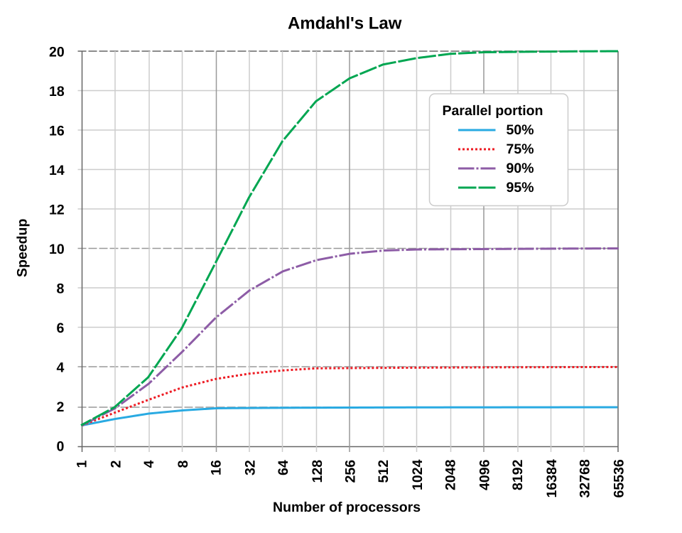 Image from Wikimedia Commons [7] (Daniels220, CC BY-SA 3.0)
The figure plots speedup against the number of processors for several parallel fractions $p$. Note that the x-axis is logarithmic. Even with $p = 0.95$ (95% parallelizable), the speedup is at most 20x. With $N = 8$ it’s $1 / (0.05 + 0.95/8) \approx 5.9$x, a parallel efficiency $S/N$ of 74%. Because the total work is fixed, the parallel part keeps shrinking as $N$ grows, while the serial part doesn’t, so the serial part takes up a larger and larger share. That’s the heart of this law.
Gustafson’s law: fix the execution time
Gustafson’s law [4], on the other hand, fixes the execution time and grows the problem size along with the number of processors $N$. In practice, when you get more processors, you usually want to solve a bigger problem (a finer mesh, a bigger model, more requests) in the same time, rather than solve the same problem faster.
This time, let the execution time on $N$ processors be 1, with a serial fraction $s$ and a parallel fraction $1 - s$. Doing that parallel work on 1 processor would take $N$ times as long, so the same amount of work would take $s + (1 - s)N$ on 1 processor. The speedup is therefore
\[S_{\text{Gustafson}}(N) = s + (1 - s)N = N - s(N - 1)\]and it keeps growing in proportion to $N$. With $s = 0.05$ and $N = 8$, it’s $8 - 0.05 \times 7 = 7.65$x.
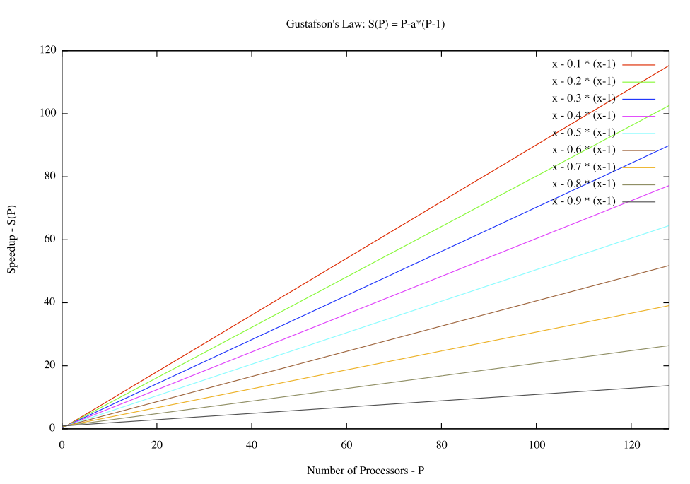 Image from Wikimedia Commons [8] (Peahihawaii, CC BY-SA 3.0)
The $a$ in the figure is the serial fraction $s$. Unlike the Amdahl figure, the x-axis here is linear, and for every $s$ the speedup grows in a straight line without leveling off.
What is held fixed?
The difference between the two formulas comes down to where you measure the serial fraction.
| Law | What’s fixed | Where the fraction is measured | Speedup as $N \to \infty$ |
|---|---|---|---|
| Amdahl | Problem size (total work) | Parallel fraction $p$ of the run time on 1 processor | Levels off at $1/(1-p)$ |
| Gustafson | Execution time (= work per processor) | Serial fraction $s$ of the run time on $N$ processors | Grows in proportion to $N$ |
In Gustafson’s setting the problem size grows with $N$, so if you imagine running it on 1 processor, the serial fraction keeps getting smaller. You can also put it this way: the $p$ you plug into Amdahl’s formula approaches 1 as $N$ grows. Neither law is “the right one”. Which formula you use depends on whether you want to solve the same problem faster, or a bigger problem in the same time.
Strong scaling and weak scaling
The ways of measuring that correspond to these two laws are strong scaling and weak scaling. Whenever a paper or benchmark claims scalability, always check which one it measured.
Strong scaling fixes the total problem size and increases the number of processors. This is Amdahl’s world. Ideally the execution time drops to $1/N$, and the parallel efficiency is
\[E_{\text{strong}}(N) = \frac{T(1)}{N \cdot T(N)}\]In LLM serving terms, it’s the situation where you take decode for the same batch, split it from 1 GPU across 8 with tensor parallelism, and want each step to take less time. In the previous post, when I estimated that running a 1T-parameter dense model on 21 machines gives 21x the bandwidth, I was assuming ideal strong scaling.
Weak scaling fixes the problem size per processor and increases the number of processors. This is Gustafson’s world. Ideally the execution time stays constant, and the parallel efficiency is
\[E_{\text{weak}}(N) = \frac{T(1)}{T(N)}\]Here $T(N)$ is the time to solve an $N$-times-larger problem on $N$ processors. Training with data parallelism at a fixed per-GPU batch size, or serving requests with an independent replica on each GPU, falls into this category.
In general, weak scaling gives better-looking numbers, and strong scaling is harder. In strong scaling, the work per processor shrinks as $N$ grows, so fixed costs like the ones we saw in the post before last (kernel launches and so on) and the communication discussed next take up a larger share.
A finer model that includes communication
Amdahl’s law only considers a serial part and a parallel part, but real parallel programs also pay for communication, and that cost changes with $N$. So let’s write the execution time as
\[T(N) = T_{\text{serial}} + \frac{T_{\text{parallel}}}{N} + T_{\text{comm}}(N)\]For example, tensor-parallel decode needs an all-reduce in every layer. With a ring all-reduce, each GPU transfers $2D(N-1)/N$ for data of size $D$, which barely goes down as $N$ grows. On top of that comes latency proportional to the number of all-reduce steps. So while $T_{\text{parallel}}/N$ shrinks as $N$ grows, $T_{\text{comm}}(N)$ stays flat or grows, which means $T(N)$ hits a minimum somewhere, and adding more GPUs beyond that point actually makes things slower. For batch-size-1 decode, each layer only takes a few tens of µs of compute, so even an all-reduce of a few µs to a dozen or so µs quickly becomes significant.
Bounding things with Amdahl’s law and then adding terms for communication and fixed costs is the same style of modeling as the per-kernel build-up from the previous post.
Computing peak performance yourself
In the earlier posts, I used peak performance numbers like 7.1 TFLOPS and 494 TFLOPS straight from the catalog specs. But where do those numbers come from? Instead of taking catalog numbers on faith, being able to compute them from the hardware configuration helps in situations like these:
- When you want the performance for a precision (FP64, INT8, etc.) or an arithmetic unit that the catalog doesn’t list
- When you want the ceiling for a program that only uses 1 core or 1 SM (comparing the naive implementation against the 99.2 GFLOPS single-core peak in the post before last was exactly this)
- When the actual operating frequency differs from the catalog value
- When the catalog doesn’t list CPU peak performance at all, which is common (that’s what “calculated” meant in the tables in previous posts)
The derivation below follows the slides of the University of Tokyo course “Parallel and Distributed Programming” [5].
CPU
CPU peak performance is
\[\text{peak performance} = \text{SIMD width} \times \text{instructions/cycle/core} \times \text{freq} \times \text{cores}\]In words: an instruction processes SIMD-width elements at once, a core can issue some number of these per cycle, there are some number of cycles per second, and there are some number of cores. Multiply them together. For FLOPS, the instruction that does the most arithmetic is the FMA (Fused Multiply Add), $d = a \times b + c$, which is 2 FLOP per element (a multiply and an add). So
\[\text{peak FLOPS} = (2 \times \text{SIMD width}) \times \text{FMA insts/cycle/core} \times \text{freq} \times \text{cores}\]GH200’s Grace uses Arm Neoverse V2 cores, each with four 128-bit SIMD pipelines, and each pipeline can issue an FMA every cycle. In FP32, 4 elements fit in 128 bits, so the SIMD width is 4. The frequencies are listed in the GH200 datasheet [6]: base frequency 3.1 GHz, all-core SIMD frequency 3.0 GHz. Using the 3.1 GHz base frequency,
\[\begin{aligned} \text{1 core} &= (2 \times 4) \times 4 \times 3.1\,\text{G} = 99.2\,\text{GFLOPS} \\ \text{72 cores} &= 99.2\,\text{GFLOPS} \times 72 \approx 7.1\,\text{TFLOPS} \end{aligned}\]and that’s where the 7.1 TFLOPS I’ve been using comes from. However, the frequency when all 72 cores keep running SIMD instructions is given as 3.0 GHz, so for a computation like matmul that saturates FMA on every core, the more accurate ceiling is
\[(2 \times 4) \times 4 \times 3.0\,\text{G} \times 72 \approx 6.9\,\text{TFLOPS}\]That said, the difference is only about 3%, so the arguments in the earlier posts still hold. For a naive implementation using only 1 core, the ceiling of 99.2 GFLOPS at 3.1 GHz is fine as is. For FP64 the SIMD width is 2, so the numbers halve to 3.6 TFLOPS and 3.5 TFLOPS respectively.
The formula also tells you something. Code that only uses scalar FMA without SIMD instructions can reach at most $1/4$ of peak (in FP32). Code that issues multiplies and adds separately instead of using FMA can reach at most half. The naive implementation in the post before last reached only about 4% of single-core peak, and on top of the memory problem, factors like these stack up.
GPU (CUDA Core)
The same idea applies to GPUs. Instead of SIMD instructions, a GPU has a warp of 32 threads execute the same instruction together. So the warp width (32) plays the role of the SIMD width, and an SM plays the role of a core. (Really, this is no surprise, since SIMT (Single Instruction, Multiple Threads), the GPU’s execution model, is an extension of SIMD that lets you write each SIMD lane as a thread [10].)
\[\text{peak FLOPS} = (2 \times \text{warp width}) \times \text{warps/cycle/SM} \times \text{freq} \times \text{SMs}\]An H100 SM is split into 4 sub-partitions, and each can execute one warp’s worth (32 lanes) of FP32 FMA per cycle (this is why people say an SM has 128 FP32 cores). So warps/cycle/SM = 4, and there are 132 SMs.
Unlike the CPU’s, the GPU frequency isn’t in the GH200 datasheet [6], but the max boost clock of the GH200’s GPU is 1980 MHz [9]. I checked on my own GH200 and got 1980 MHz as well.
$ nvidia-smi --query-gpu=clocks.max.sm --format=csv
clocks.max.sm [MHz]
1980 MHz
Using this,
\[(2 \times 32) \times 4 \times 1.98\,\text{G} \times 132 \approx 66.9\,\text{TFLOPS}\]which gives the 67 TFLOPS in the spec table.
GPU (Tensor Core)
A Tensor Core is an arithmetic unit that computes a small matrix multiply in a single instruction. Each H100 Tensor Core can compute $C = A \times B + C$ once per cycle, with TF32 inputs $A$ ($4 \times 8$) and $B$ ($8 \times 8$) and FP32 $C$ [5]. Each of the $4 \times 8$ outputs is a length-8 dot product (8 FMAs), so the work per cycle is
\[2 \times 4 \times 8 \times 8 = 512\,\text{FLOP/cycle}\]Each H100 SM has 4 Tensor Cores, so 132 SMs give $4 \times 132 = 528$ Tensor Cores. At the same 1.98 GHz,
\[512\,[\text{FLOP/cycle}] \times 1.98\,\text{G}\,[\text{cycle/s}] \times 528\,[\text{Tensor Cores}] \approx 535.3\,\text{TFLOPS}\]Per SM, CUDA Cores do 256 FLOP/cycle while Tensor Cores do $512 \times 4 = 2048$ FLOP/cycle, 8 times as much. That’s why using Tensor Cores is fast.
Going to lower precision, the number of elements processed per cycle grows in inverse proportion to the precision, giving 1070.5 TFLOPS for FP16/BF16 and 2141.1 TFLOPS for FP8 (all dense). Every value computed here is for dense matmul. Catalogs sometimes list values using 2:4 structured sparsity alongside, and those are twice the dense values, so watch out.
The formula predicts quite accurately
Let’s put these results next to the values in the datasheet [6].
| Unit | Formula (1.98 GHz) | Datasheet | Datasheet / Formula |
|---|---|---|---|
| CUDA Core FP32 | 66.9 TFLOPS | 67 TFLOPS | 1.00 |
| Tensor Core TF32 | 535.3 TFLOPS | 494 TFLOPS | 0.92 |
| Tensor Core BF16 | 1070.5 TFLOPS | 990 TFLOPS | 0.92 |
| Tensor Core FP8 | 2141.1 TFLOPS | 1,979 TFLOPS | 0.92 |
For CUDA Cores, the formula gives exactly the datasheet value. For Tensor Cores, the datasheet is about 8% lower, but the thing to notice is that the ratio is 0.92 for TF32, BF16 and FP8 alike. The only term in the formula that changes with precision is the work per cycle, so a constant ratio means the gap doesn’t come from there. It comes from a term shared by all precisions: the frequency. NVIDIA doesn’t state the reason, but presumably it’s because high-power workloads that saturate the Tensor Cores can’t sustain the max boost clock, so the Tensor Core numbers are quoted at a lower frequency.
So peak performance can be predicted quite accurately as the product of a few factors: SIMD width, instructions per cycle, frequency, and core count. And when a prediction is off, you can narrow down which factor is off.
This is useful because when measured performance falls short of the theoretical FLOPS, you can break it down and analyze which factor is missing. If all you have is the catalog number of 494 TFLOPS, you can’t say anything beyond “I’m only getting 80%”. But once you break it into the formula, you can split the problem into hypotheses you can check one at a time:
- Frequency: is the clock dropping during the measurement?
- SIMD width: are SIMD or Tensor Core instructions actually being used (or has it fallen back to scalar instructions or CUDA Cores)?
- Instructions per cycle: is it using FMA, and is it issuing an instruction every cycle?
- Core count: is work being assigned to every core or SM?
In the next section, I’ll go into frequency, which is the easiest of these to overlook.
Frequency isn’t constant
Just as the Tensor Core datasheet values were lower than the values computed at the max boost clock, on the CPU side the Grace datasheet lists an all-core SIMD frequency (3.0 GHz) separately from the base frequency (3.1 GHz). That’s because keeping the SIMD units busy on every core makes the frequency drop due to power limits.
Both GPUs and CPUs change their operating frequency dynamically depending on power and temperature. There’s no guarantee they actually run at the frequency in the datasheet or spec table.
In other words, frequency is the most uncertain term in the theoretical peak formula. When you run experiments, it’s worth checking the actual frequency.
# GPU: current clock and max clock
nvidia-smi --query-gpu=clocks.sm,clocks.max.sm --format=csv
# Watch how the clock changes during a measurement
nvidia-smi dmon -s pc
# CPU
lscpu | grep -i mhz
If the clock drops to 1.6 GHz during a measurement, the Tensor Core TF32 ceiling is $512 \times 1.6\,\text{G} \times 528 \approx 433$ TFLOPS. In the post before last, PyTorch’s TF32 matmul reached 399 TFLOPS (81% of 494 TFLOPS), but compared against a ceiling recomputed at the actual frequency, the achieved fraction might be even higher. Conversely, if you don’t notice that the frequency has dropped, you may blame your implementation and keep hunting for headroom that doesn’t exist.
The catalog number of 494 TFLOPS alone can’t tell you “it was because the frequency dropped”. Estimating peak performance from the formula lets you dig into factors like frequency when you’re not reaching theoretical FLOPS, and that’s the main reason not to stop at the spec values.
Summary
- Amdahl’s law is the speedup when the problem size is fixed. It levels off at $1/(1-p)$ because of the serial fraction $1-p$. It corresponds to strong scaling.
- Gustafson’s law is the speedup when the execution time (work per processor) is fixed. It grows in proportion to $N$. It corresponds to weak scaling.
- In real parallel programs, terms for communication and fixed costs change with $N$. Adding them to the model lets you estimate the point where adding GPUs stops helping.
- Peak performance can be computed as $(2 \times \text{SIMD width}) \times \text{FMA insts/cycle/core} \times \text{freq} \times \text{cores}$. For GPUs you swap in the warp width and SM count, and for Tensor Cores the matmul size per cycle. This formula reproduces the datasheet values quite accurately.
- Once you break it into the formula, you can analyze whether frequency, SIMD, FMA or core count is the cause when you’re not reaching theoretical FLOPS.
- Frequency is the term that varies the most. The H100 Tensor Core datasheet values are computed at a frequency below the max boost clock, and Grace has a separate frequency for SIMD. Check the actual clock during your measurements and compare against a ceiling based on it.
Reference
[1] Wikipedia, “Amdahl’s law”, https://en.wikipedia.org/wiki/Amdahl%27s_law
[2] Wikipedia, “Gustafson’s law”, https://en.wikipedia.org/wiki/Gustafson%27s_law
[3] G. M. Amdahl, “Validity of the single processor approach to achieving large scale computing capabilities”, AFIPS Spring Joint Computer Conference, 1967, https://doi.org/10.1145/1465482.1465560
[4] J. L. Gustafson, “Reevaluating Amdahl’s law”, Communications of the ACM, 1988, https://doi.org/10.1145/42411.42415
[5] K. Taura, Parallel and Distributed Programming, lecture slides “Introduction”, https://taura.github.io/parallel-distributed-programming/slides/intro.pdf
[6] NVIDIA, “NVIDIA GH200 Grace Hopper Superchip Datasheet”, 2024, https://www.nvidia.com/en-us/data-center/grace-hopper-superchip/
[7] Daniels220, “AmdahlsLaw.svg”, Wikimedia Commons, CC BY-SA 3.0, https://commons.wikimedia.org/wiki/File:AmdahlsLaw.svg

[8] Peahihawaii, “Gustafson.png”, Wikimedia Commons, CC BY-SA 3.0, https://commons.wikimedia.org/wiki/File:Gustafson.png

[9] Wikipedia, “Grace Hopper GH200”, https://en.wikipedia.org/wiki/Grace_Hopper_GH200
[10] NVIDIA, “CUDA C++ Programming Guide (v12.4), 4.1 SIMT Architecture”, https://docs.nvidia.com/cuda/archive/12.4.0/cuda-c-programming-guide/index.html#simt-architecture